1. 症例背景(既往歴・経過)
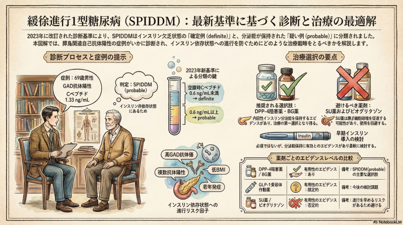
基本属性: 69歳の男性です。糖尿病の経過: 14年前に糖尿病と診断 されました。紹介時の状況: 11年前の血液検査では、抗GAD抗体陽性 (4年前の再検でも43.9 U/mLと陽性)、空腹時血清Cペプチド 1.3 ng/mL、HbA1c 6.0%でした。治療歴: これまで経口血糖降下薬やインスリンは使用せず、HbA1c 6%台前半で経過していました。併用薬: 糖尿病以外に、高脂血症や高血圧などの治療のため、ピタバスタチン、テルミサルタン、フェブキソスタットを2年間継続して服用しています。
2. 現症(身体所見・症状)
体格: 身長 173 cm、体重 67 kg、BMI 22.3 kg/m² であり、ここ数年の体重変動はありません。合併症: 糖尿病網膜症は認められません 。
3. 検査所見
血糖コントロール: HbA1c 7.8% (直近3か月間は7.0%を超えており、それ以前は7.0%未満でした)。インスリン分泌能: 空腹時血清Cペプチドは 1.33 ng/mL であり、過去2年間の推移(1.26 → 1.18 ng/mL)を見ても、内因性インスリン分泌能は保持 されています。腎機能: 尿中アルブミン/クレアチニン比は 12.6 mg/g・Crであり、基準値(30未満)内です。その他: 昨年実施した上下部内視鏡検査および腹部超音波検査では、異常は認められていません。
4. 臨床診断
この症例は、抗GAD抗体が陽性であるものの、最終観察時点での空腹時血清Cペプチドが0.6 ng/mL以上であり、内因性インスリン欠乏状態には至っていないことから、2023年の新診断基準における**「緩徐進行1型糖尿病(SPIDDM:probable)」、すなわち 緩徐進行1型糖尿病疑い例**と診断されます。
緩徐進行1型糖尿病(SPIDDM)疑い例(probable)における診療管理プロトコル:2023年改訂基準に基づく実践指針
1. 緒言:2023年改訂診断基準の戦略的意義
2023年、緩徐進行1型糖尿病(SPIDDM)の診断基準は、2012年の策定から10年以上の歳月を経て大きな転換期を迎えました。今回の改訂における最大の戦略的意義は、病態を**「definite(確定)」と 「probable(疑い)」**の2つのカテゴリーに明確に分離した点にあります。
従来の2012年基準では、インスリン依存状態への進行リスクが明らかなGAD抗体とICA(膵島細胞抗体)のみを対象としており、IA-2抗体単独陽性例などの扱いが不明確でした。また、自己抗体陽性例であっても全例が必ずしもインスリン依存状態へ進行するわけではないという知見が蓄積され、「進行リスクの多様性」への対応が急務となっていました。
「probable」というカテゴリーの新設は、インスリン非依存状態にある症例に対し、早期の一律的なインスリン導入という固定概念を脱却し、患者個々のリスクに応じた「柔軟な治療選択」と「厳密な経過観察」を両立させるために不可欠な措置です。これにより、海外のLADA概念との整合性を保ちつつ、日本の臨床実態に即した管理が可能となりました。正確な診断から管理を開始するための体系的フローを次章で整理します。
——————————————————————————–
2. 診断基準の体系的整理と「probable」の定義
SPIDDMの診断は、自己抗体の有無、発症時の病態、およびインスリン分泌能の推移という3つの軸で判定されます。専門医は以下の診断マトリクスに基づき、速やかに病態を識別する必要があります。
■ SPIDDM診断マトリクス(2023)
診断には以下の3つの必須項目を用います。
必須項目1(自己抗体): 経過のどこかで膵島関連自己抗体(GAD、ICA、IA-2、ZnT8、IAA※)のいずれかが陽性である(※IAAはインスリン治療開始前に限る)。必須項目2(非依存状態): 原則として糖尿病診断時にケトーシスがなく、直ちにインスリン療法を必要としない。必須項目3(インスリン欠乏): 糖尿病診断後3ヶ月を過ぎてインスリン療法が必要となり、最終的に内因性インスリン欠乏(空腹時血清Cペプチド < 0.6 ng/mL )となる。
注:インスリン依存状態への移行期間は、典型例では6ヶ月以上を要する。
【判定区分】
definite (確定): 項目1、2、3のすべてを満たす状態。probable (疑い): 項目1、2のみを満たし、項目3(インスリン欠乏)をまだ満たしていない状態。
■ 臨床的概念の重なり
「probable」は、海外の**LADA(latent autoimmune diabetes in adults)の主要概念を包含するものです。典型例は35歳以降の発症ですが、若年者で同様の経過をたどる症例は LADY(latent autoimmune diabetes in youth)**と呼ばれます。今回の改訂により、これら広義の自己免疫性糖尿病を「SPIDDM疑い」として国内基準で管理できるようになった意義は極めて大きいと言えます。診断確定後の次なるステップは、個々の症例の進行リスク評価です。
——————————————————————————–
3. インスリン依存状態への進行リスク評価
SPIDDM(probable)症例において、最も重要な臨床判断は「いつインスリン欠乏に至るか」の予測です。以下の指標が認められる場合は、速やかな進行が懸念される「ハイリスク群」として警戒を強める必要があります。
■ 進行を予測する主要因子
自己抗体の力価と種類:
複数抗体陽性: GAD抗体に加え、IA-2抗体やZnT8抗体が陽性である場合は、進行リスクが有意に高い(Kawasakiらの報告)。GAD 抗体価: 従来のRIA法では高力価(≧10 U/mL)がリスク因子でした。現行のELISA法については結論を待つ段階ですが、高値維持例には注意を要します。【エキスパート・パール:保険診療上の制限】 現在の日本の保険制度上、GAD抗体陽性が確認された場合、IA-2抗体やZnT8抗体の測定は保険適用外 となる点に注意してください。リスク評価のための追加測定には、この制度的制約を念頭に置く必要があります。
併存疾患と多発性自己免疫:
抗TPO抗体陽性(Ehime Study): 甲状腺自己抗体である抗TPO抗体陽性は、膵β細胞機能不全(beta cell failure)への進行リスクを高めます。これは、本病態が「多発性自己免疫(polyautoimmunity)」の一環として進行している可能性を示唆する重要な所見です。
患者背景:
若年発症(45歳以下)、低BMI、診断時の低Cペプチド値: これらは国内外の研究(UKPDS等)で共通して指摘されている進行加速因子です。
これらのリスク評価の結果は、次章で詳述する薬剤選択における優先順位の決定要因となります。
——————————————————————————–
4. 薬剤選択の論理的根拠と禁忌指針
SPIDDM(probable)はインスリン非依存状態であるため、膵β細胞保護を最大化する戦略的薬剤選択が求められます。当委員会は、エビデンスに基づき以下のカテゴリー分類を推奨します。
■ 回避すべき薬剤:SU(スルホニル尿素)薬
【評価:原則回避】 Tokyo study により、SU薬の使用はインスリン療法と比較して内因性インスリン分泌能の低下を有意に促進することが示されました。
メカニズム(Impact): SU薬による過度なβ細胞刺激が、膵島における抗原提示を促進 し、免疫担当細胞によるβ細胞破壊を加速させると推察されています。
■ 治療選択肢の体系化(Fig. 1のカテゴリーに基づく)
① 有用性に関するエビデンスがある薬剤(推奨)
DPP-4 阻害薬: 国内のSPAN-S研究 等により、内因性インスリン分泌能を保持する可能性が示唆されています。膵島へのリンパ球浸潤抑制効果も期待され、臨床的妥当性が極めて高い選択肢です。ビグアナイド(BG)薬: パイロット研究において、ピオグリタゾンよりも分泌能保持に寄与する可能性が示されています。腸内細菌叢を介した免疫調整能の観点からも、使用を妨げる根拠はありません。インスリン療法: 早期導入により膵β細胞を休養させ、分泌能を保持するエビデンスがあります。ただし、現在のコンセンサスでは「全例必須」ではなく、低リスク例では他の経口薬との選択になります。
② 有用性に関するエビデンスが限定的な薬剤
GLP-1 受容体作動薬: HbA1c改善効果は認められますが、分泌能保持に関するSPIDDM特異的なエビデンスはまだ不十分です。
③ 推奨されない、または見解がない薬剤
ピオグリタゾン(非推奨): 他の薬剤に比べ、内因性インスリン分泌能を保持できない可能性が指摘されています。SGLT2 阻害薬、α-GI、グリニド薬、イメグリミン: 現時点でSPIDDMに対する見解(エビデンス)はありません。
薬剤選択後は、その成否を判断するための厳格な監視体制へ移行します。
——————————————————————————–
5. 内因性インスリン分泌能の監視と治療強化プロトコル
治療開始後は、病態の「進行」を早期に捉えるため、当委員会は以下のモニタリングフローの遵守を推奨します。
■ 監視アクションプラン(Protocol Flow)
定期評価(3〜6ヶ月毎): HbA1cによる血糖管理指標の確認に加え、**空腹時血清Cペプチド(CPR)**の定期測定をルーチン化してください。進行傾向の検知: HbA1cの悪化、あるいはCPR値が徐々に低下する「低下トレンド」を認めた場合は、内因性インスリン分泌能の減衰と判断します。治療強化・インスリン転換の実施: 分泌能低下が疑われた際は、経口薬に固執せず、**躊躇なく速やかなインスリン治療への変更(または強化)**を行ってください。これが、完全なインスリン依存状態への移行を食い止めるための最終的な介入閾値となります。長期的合併症評価: 中長期的な視点から、網膜症や腎症などの血管合併症の進展評価を並行して実施してください。
——————————————————————————–
6. 保険診療上の対応と運用の実際
日本国内での実務上、SPIDDM(probable)の管理には制度面への配慮が不可欠です。
病名の運用の現状: 現在、DPP-4阻害薬やビグアナイド薬は、保険診療上の「1型糖尿病」病名に対して適用がありません。そのため、インスリン非依存状態であるprobable例に対してこれらの薬剤を処方する際は、暫定的な必要置置として「NIDDM(2型糖尿病)」の病名を併記するなどの対応 が求められます。今後の課題: 「緩徐進行1型糖尿病疑い」という適切な病名で、エビデンスのある薬剤が円滑に使用できるよう、審査体制や制度の整備について今後も議論を継続していく必要があります。
——————————————————————————–
7. 総括:膵β細胞保護を最大化するマネジメント
SPIDDM(probable)の管理における至上命題は、**「内因性インスリン分泌能の枯渇(Cペプチド < 0.6 ng/mL)をいかに遅らせ、患者のQOLを維持するか」**にあります。2023年の改訂診断基準を武器に、確定診断前の「疑い」段階から戦略的に介入することが、長期予後を左右します。
柔軟な薬剤選択と、一転して厳格な分泌能モニタリングという二段構えのマネジメントこそが、将来的なインスリン依存状態への進行抑制に直結するのです。
■ 主要な推奨事項
SU 薬の使用は、抗原提示を促進しβ細胞破壊を加速させる恐れがあるため、厳に避けること。 薬剤選択は、カテゴリー①に分類されるDPP-4阻害薬、BG薬、またはインスリン療法を優先すること。 空腹時Cペプチド測定を定期評価に組み込み、HbA1cのみでは見えない「分泌能の低下傾向」を捉えること。 分泌能の低下を認めた場合は、速やかにインスリン治療への転換(または追加)という治療強化を行うこと。 保険診療上の制約(IA-2抗体測定制限や病名運用)を正しく理解し、個々の患者に最適な個別化医療を実践すること。
Podcast: Play in new window | Download