CMPRSKパッケージとは
{cmprsk} は、競合リスクイベントのある生存時間分析を実施するためのRパッケージです1。具体的には、次の3つの機能を持っています:
- 群間の累積発生関数 (Cumulative Incidence Function; CIF) の同等性の比較検定 (Gray’s test): 異なる群の間でCIFの同等性を比較します。
- 推定されたCIFを表として出力する機能: 群ごとに推定されたCIFを表形式で表示します。
- 推定されたCIFをグラフとして出力する機能: 群ごとに推定されたCIFをグラフで視覚化します。
このパッケージは、Luca Scrucca氏による{cmprsk}パッケージに基づくラッパー関数であり、詳細な解説は本人のサイトで提供されています1。
使用法と主な引数は以下の通りです:
ftime: 生存期間 (failure time variable)fstatus: 発生したイベントを示すコード (variable with distinct codes for different causes of failure and also a distinct code for censored observations)group: 比較する群を指定するコード (estimates will be calculated within groups given by distinct values of this variable)t: CIFを評価する時点を指定するベクトル (a vector of time points where the cumulative incidence function should be evaluated)strata: 層別化して検定を実施したい場合に指定する、層を示す変数 (stratification variable)- その他のオプション引数:
rho, cencode, subset, na.action, level, xlab, ylab, col, lty, lwd, digits など
このパッケージを使って、競合リスクイベントのある生存時間データを効果的に分析できます
スクリプト
library(cmprsk)

# Fits the ’proportional subdistribution hazards’ regression model described in Fine and Gray (1999).
# This model directly assesses the effect of covariates on the subdistribution of a particular type of
# failure in a competing risks setting. The method implemented here is described in the paper as the
# weighted estimating equation.
# While the use of model formulas is not supported, the model.matrix function can be used to gener-
#   ate suitable matrices of covariates from factors, eg model.matrix(~factor1+factor2)[,-1] will
# generate the variables for the factor coding of the factors factor1 and factor2. The final [,-1]
# removes the constant term from the output of model.matrix.
# The basic model assumes the subdistribution with covariates z is a constant shift on the complemen-
#   tary log log scale from a baseline subdistribution function. This can be generalized by including
# interactions of z with functions of time to allow the magnitude of the shift to change with follow-up
# time, through the cov2 and tfs arguments. For example, if z is a vector of covariate values, and uft is
# a vector containing the unique failure times for failures of the type of interest (sorted in ascending
#                                                                                    order), then the coefficients a, b and c in the quadratic (in time) model az + bzt + zt2 can be fit by
# specifying cov1=z, cov2=cbind(z,z), tf=function(uft) cbind(uft,uft*uft).
# This function uses an estimate of the survivor function of the censoring distribution to reweight
# contributions to the risk sets for failures from competing causes. In a generalization of the method-
#   ology in the paper, the censoring distribution can be estimated separately within strata defined by
# the cengroup argument. If the censoring distribution is different within groups defined by covari-
#   ates in the model, then validity of the method requires using separate estimates of the censoring
# distribution within those groups.
# The residuals returned are analogous to the Schoenfeld residuals in ordinary survival models. Plot-
#   ting the jth column of res against the vector of unique failure times checks for lack of fit over time
# in the corresponding covariate (column of cov1).
# If variance=FALSE, then some of the functionality in summary.crr and print.crr will be lost.
# This option can be useful in situations where crr is called repeatedly for point estimates, but standard
# errors are not required, such as in some approaches to stepwise model selection.

# simulated data to test
set.seed(10)
ftime <- rexp(200)
fstatus <- sample(0:2,200,replace=TRUE)
cov <- matrix(runif(600),nrow=200)
dimnames(cov)[[2]] <- c('x1','x2','x3')
print(z <- crr(ftime,fstatus,cov))
summary(z)
z.p <- predict(z,rbind(c(.1,.5,.8),c(.1,.5,.2)))
plot(z.p,lty=1,color=2:3)
crr(ftime,fstatus,cov,failcode=2)
# quadratic in time for first cov
crr(ftime,fstatus,cov,cbind(cov[,1],cov[,1]),function(Uft) cbind(Uft,Uft^2))
#additional examples in test.R
以下にスクリプトの機能とそれぞれの部分の説明を提供します。
- ライブラリの読み込み:
library(cmprsk): {cmprsk}パッケージを読み込みます。
- シミュレートされたデータの作成:
set.seed(10): 乱数生成のシードを設定します。ftime <- rexp(200): 200個の指数分布からなる生存時間データを生成します。fstatus <- sample(0:2,200,replace=TRUE): 200個のランダムなイベントコード(0, 1, 2)を生成します。cov <- matrix(runif(600),nrow=200): 200行3列の乱数行列を生成します。dimnames(cov)[[2]] <- c('x1','x2','x3'): 列名を ‘x1’, ‘x2’, ‘x3’ に設定します。
- crr関数を使用して競合リスクイベントのある生存時間データを分析:
z <- crr(ftime,fstatus,cov): 群間の累積発生関数(CIF)の同等性を比較し、推定されたCIFを表として出力します。summary(z): 分析結果のサマリーを表示します。z.p <- predict(z,rbind(c(.1,.5,.8),c(.1,.5,.2))): 推定されたCIFを指定した時点で計算し、結果を表示します。plot(z.p,lty=1,color=2:3): 推定されたCIFをグラフで表示します。crr(ftime,fstatus,cov,failcode=2): 特定の失敗コードを持つデータを用いて再度分析を実行します。crr(ftime,fstatus,cov,cbind(cov[,1],cov[,1]),function(Uft) cbind(Uft,Uft^2)): 最初の共変量に対して時間の2次項を考慮した分析を実行します。
- 追加の例:
test.Rファイルにさらなる例が含まれています。
このスクリプトは、競合リスクイベントのある生存時間データの解析に役立ちます。詳細な使い方やパラメータの調整については、{cmprsk}パッケージのドキュメントや解説を参照してください 123。
# 実行結果
> print(z <- crr(ftime,fstatus,cov))
convergence: TRUE
coefficients:
x1 x2 x3
0.26680 -0.05568 0.28050
standard errors:
[1] 0.4211 0.3812 0.3810
two-sided p-values:
x1 x2 x3
0.53 0.88 0.46
> summary(z)
Competing Risks Regression
Call:
crr(ftime = ftime, fstatus = fstatus, cov1 = cov)
coef exp(coef) se(coef) z p-value
x1 0.2668 1.306 0.421 0.633 0.53
x2 -0.0557 0.946 0.381 -0.146 0.88
x3 0.2805 1.324 0.381 0.736 0.46
exp(coef) exp(-coef) 2.5% 97.5%
x1 1.306 0.766 0.572 2.98
x2 0.946 1.057 0.448 2.00
x3 1.324 0.755 0.627 2.79
Num. cases = 200
Pseudo Log-likelihood = -320
Pseudo likelihood ratio test = 1.02 on 3 df,
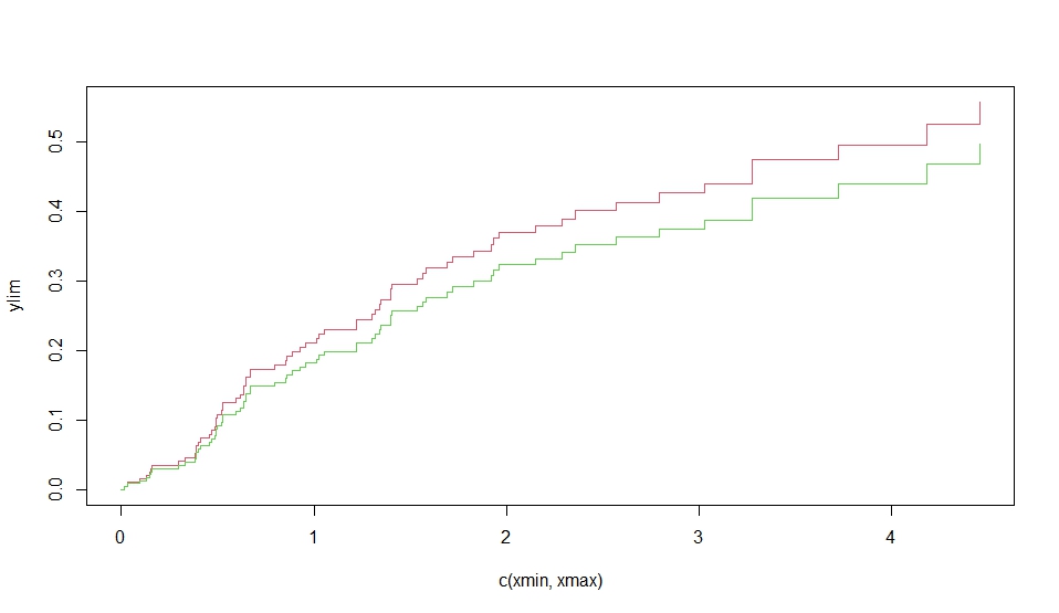
> z.p <- predict(z,rbind(c(.1,.5,.8),c(.1,.5,.2)))
> plot(z.p,lty=1,color=2:3)
> crr(ftime,fstatus,cov,failcode=2)
convergence: TRUE
coefficients:
x1 x2 x3
-0.31390 -0.03488 -0.52500
standard errors:
[1] 0.4517 0.4475 0.4675
two-sided p-values:
x1 x2 x3
0.49 0.94 0.26
> # quadratic in time for first cov
> crr(ftime,fstatus,cov,cbind(cov[,1],cov[,1]),function(Uft) cbind(Uft,Uft^2))
convergence: TRUE
coefficients:
x1 x2 x3
2.16500 -0.06664 0.27490
cbind(cov[, 1], cov[, 1])1*Uft cbind(cov[, 1], cov[, 1])2*tf2
-3.25200 0.81900
standard errors:
[1] 0.9464 0.3797 0.3854 1.2590 0.2925
two-sided p-values:
x1 x2 x3
0.0220 0.8600 0.4800
cbind(cov[, 1], cov[, 1])1*Uft cbind(cov[, 1], cov[, 1])2*tf2
0.0098 0.0051
次に、Rの cmprsk パッケージを使用して、競合リスク(competing risks)の累積発生率を比較するための解析を行っています。
############################
set.seed(2)
ss <- rexp(100)
gg <- factor(sample(1:3,100,replace=TRUE),1:3,c('a','b','c'))
cc <- sample(0:2,100,replace=TRUE)
strt <- sample(1:2,100,replace=TRUE)
print(xx <- cuminc(ss,cc,gg,strt))
plot(xx,lty=1,color=1:6)
# see also test.R, test.out
具体的には、次の手順を実行しています:
- データの生成:
set.seed(2) で乱数のシードを設定しています。rexp(100) で指数分布に従うランダムなイベント時間を生成しています。sample(1:3, 100, replace=TRUE) でランダムなイベントの状態(3つのグループ ‘a’, ‘b’, ‘c’)を生成しています。sample(0:2, 100, replace=TRUE) でランダムな検閲状態(0, 1, 2)を生成しています。sample(1:2, 100, replace=TRUE) でランダムな開始時点を生成しています。
cuminc 関数の実行:
cuminc(ss, cc, gg, strt) で競合リスクの累積発生率を計算しています。ss はイベント時間、cc はイベントの状態、gg はグループ、strt は開始時点です。
- 結果の表示:
print(xx) で計算された累積発生率を表示しています。
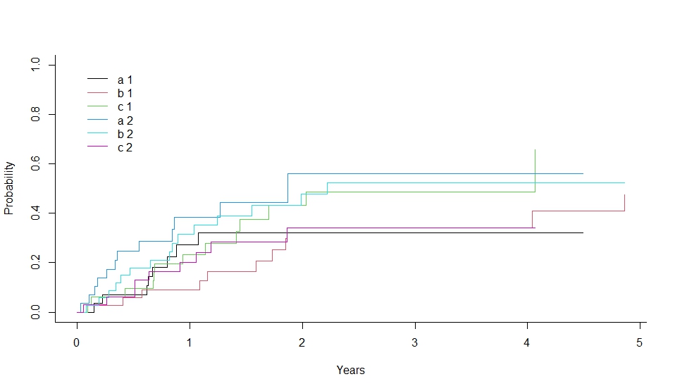
- グラフの描画:
plot(xx, lty=1, color=1:6) で累積発生率のグラフを描画しています。
############################
set.seed(2)
ss <- rexp(100)
gg <- factor(sample(1:3,100,replace=TRUE),1:3,c(‘a’,’b’,’c’))
cc <- sample(0:2,100,replace=TRUE)
strt <- sample(1:2,100,replace=TRUE)
print(xx <- cuminc(ss,cc,gg,strt))
plot(xx,lty=1,color=1:6)
# see also test.R, test.out
############################
set.seed(2)
ss <- rexp(100)
gg <- factor(sample(1:3,100,replace=TRUE),1:3,c('a','b','c'))
cc <- sample(0:2,100,replace=TRUE)
strt <- sample(1:2,100,replace=TRUE)
print(xx <- cuminc(ss,cc,gg,strt))
plot(xx,lty=1,color=1:6)
# see also test.R, test.out
このコードは、競合リスクの解析において、各グループの累積発生率を比較するための有用な手法を示しています。12
詳細については、公式ドキュメントをご参照ください:cmprsk パッケージ1。
> print(xx <- cuminc(ss,cc,gg,strt))
Tests:
      stat        pv df
1 1.598854 0.4495865  2
2 3.390543 0.1835493  2
Estimates and Variances:
$est
             1         2         3         4
a 1 0.27262599 0.3216446 0.3216446 0.3216446
b 1 0.08877315 0.3423257 0.3423257 0.3423257
c 1 0.23368736 0.4312495 0.4879272 0.4879272
a 2 0.38424403 0.5607109 0.5607109 0.5607109
b 2 0.31463271 0.4786961 0.5234407 0.5234407
c 2 0.20127996 0.3420399 0.3420399 0.3420399

$var
              1           2           3           4
a 1 0.008596053 0.009950848 0.009950848 0.009950848
b 1 0.002491270 0.009675072 0.009675072 0.009675072
c 1 0.006341967 0.011566190 0.012617195 0.012617195
a 2 0.010293273 0.022358101 0.022358101 0.022358101
b 2 0.007220502 0.010014466 0.010588994 0.010588994
c 2 0.005699657 0.010260038 0.010260038 0.010260038